SAR (Synthetic-Aperture Radar) [2024.11.13]
Synthetic-aperture radar imagery of the sea surface from Sentinel-1, ERS and ALOS, with download routes (ASF, Copernicus Data Space) and MATLAB tools.
About SAR
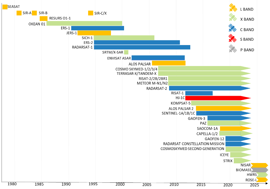
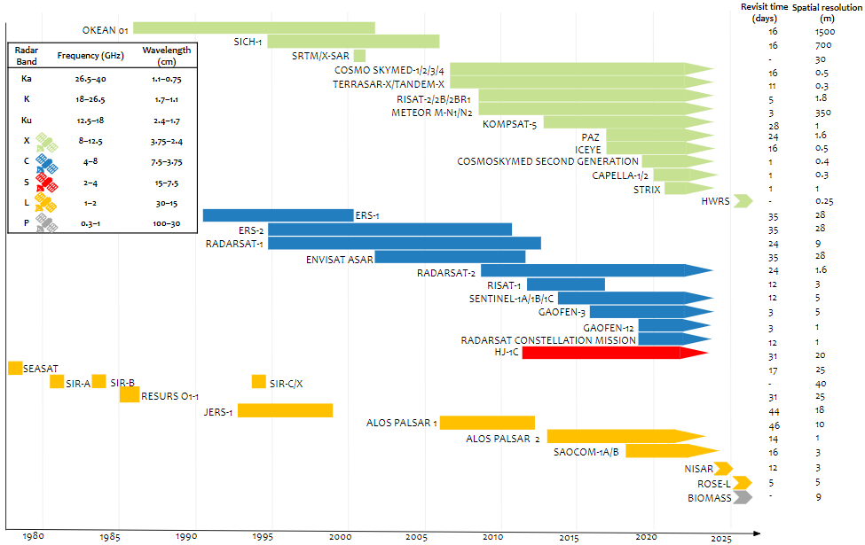
About Sentinel-1
Sentinel-1 is the first of the Copernicus Programme satellite constellations conducted by the European Space Agency. The mission was originally composed of a constellation of two satellites, Sentinel-1A and Sentinel-1B, which shared the same orbital plane. Sentinel-1A was launched on 3 April 2014, and Sentinel-1B on 25 April 2016. (Wikipedia)
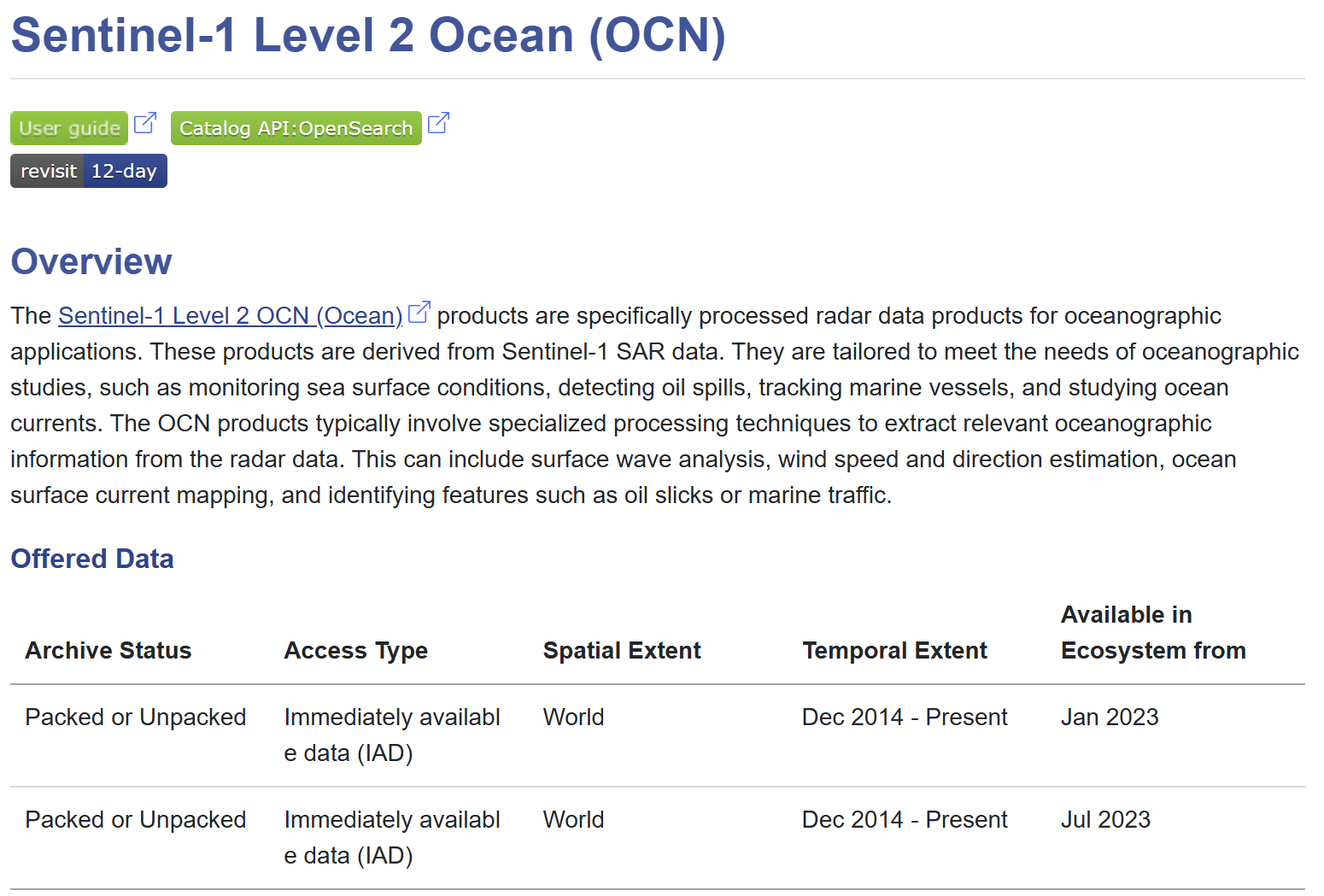
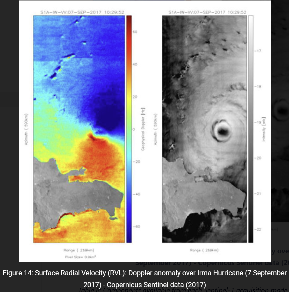
Sentinel-1 normally observes wide areas at low resolution and switches to high-resolution, narrow-swath modes over regions of interest. Its strength is that it is weather-independent; its weaknesses are that interpretation is difficult and, above all, that coverage of the ocean is limited (coastal acquisitions exist, but open-sea acquisitions are few).
MATLAB tools
- oceanremotesensing/MATLAB_SAR
- SAR Processor (File Exchange)
- SAR Signal Processing with MATLAB Algorithms, Reloaded (File Exchange)
Download from ASF (ERS, Sentinel-1, ALOS)
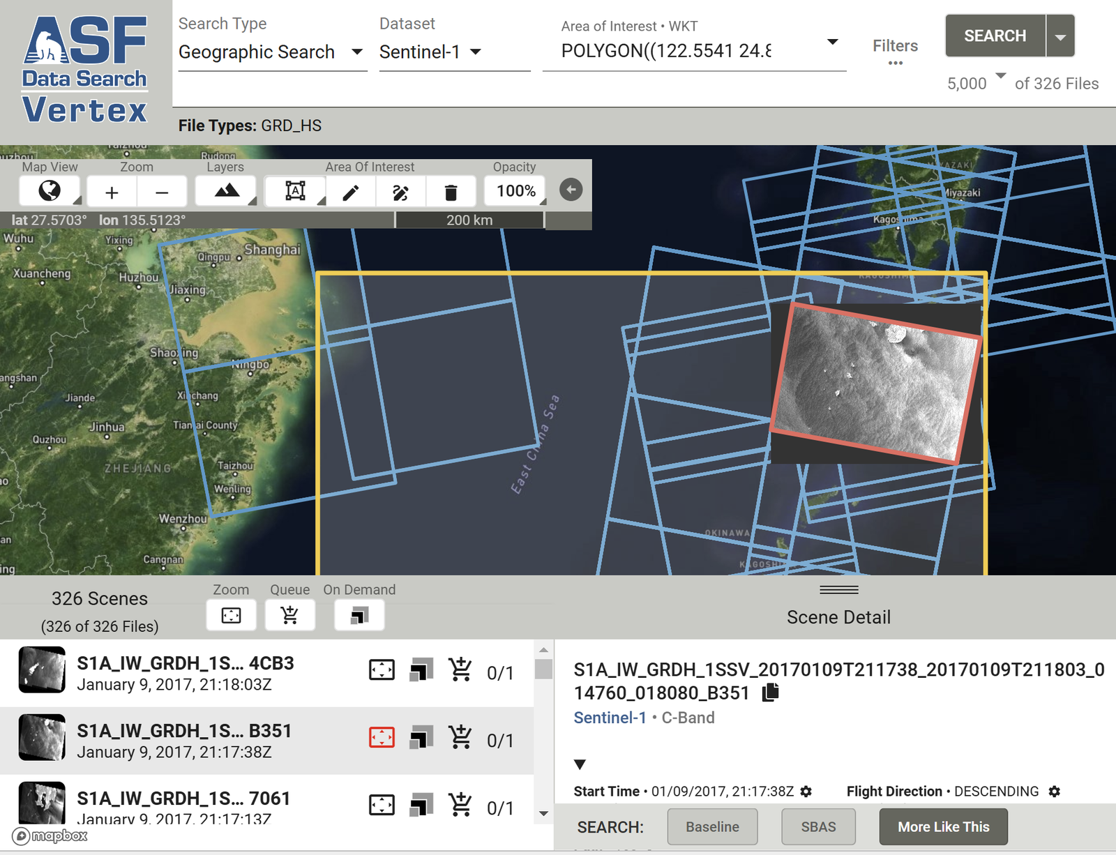
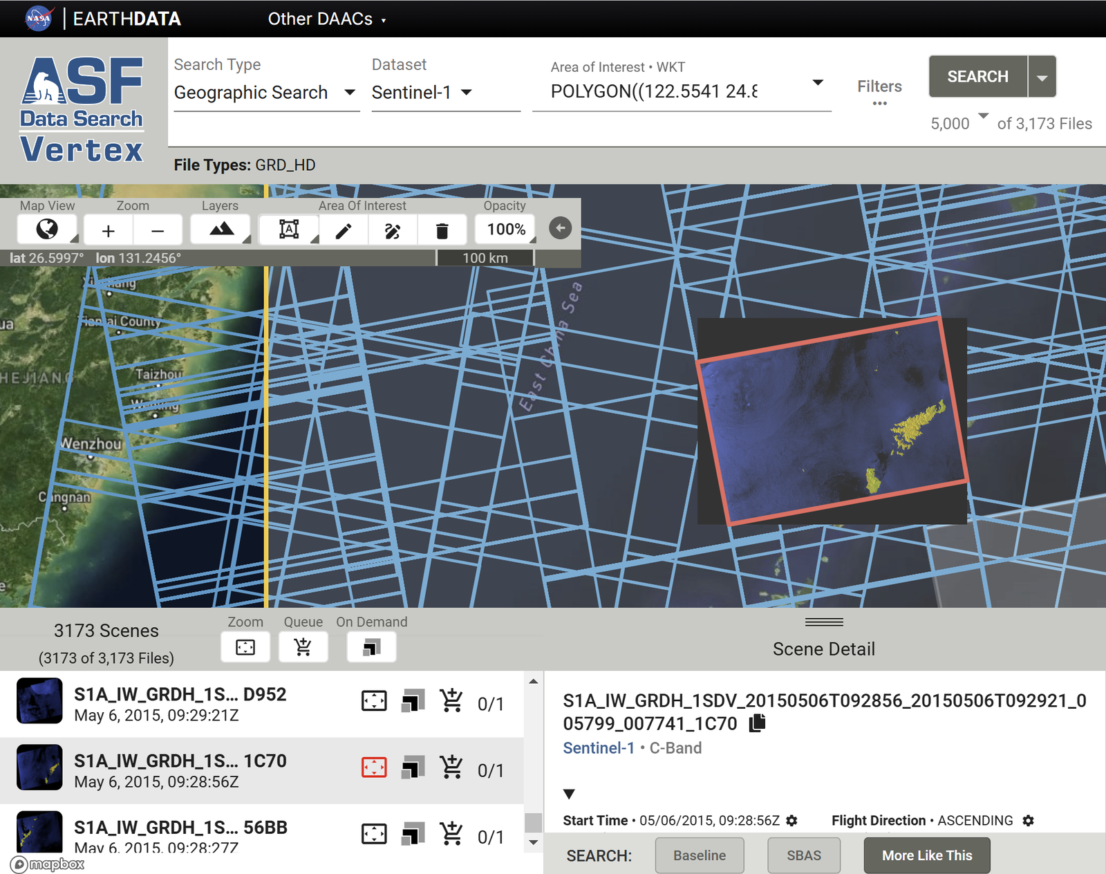
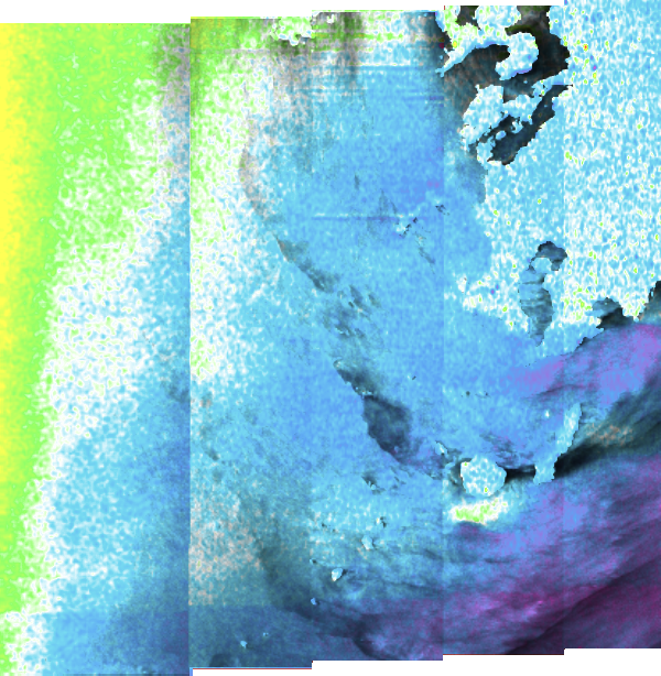
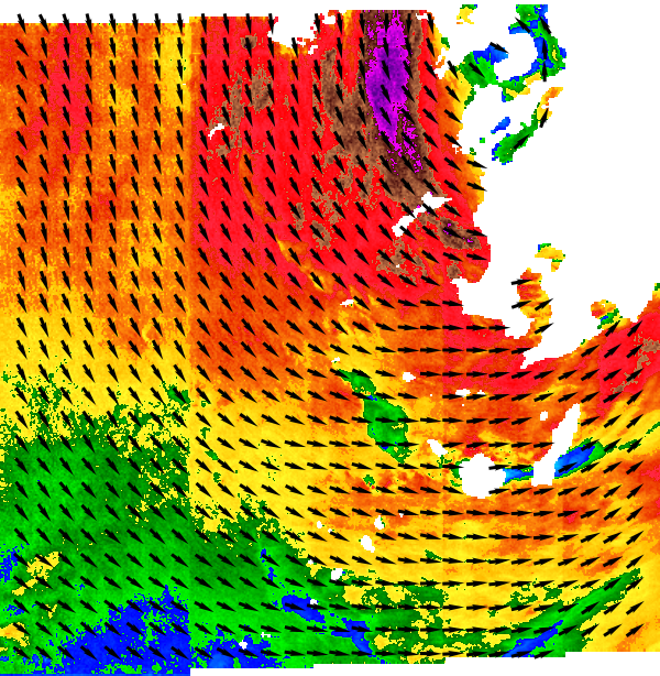
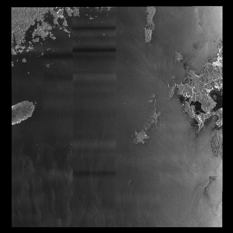
GRD_HS and GRD_HD products can be previewed in Vertex, but OCN products cannot; OCN can only be checked after download. The example below shows OCN data for the East China Sea, southwest of Kyushu.
ALOS data from Japan can be downloaded the same way. The example below covers the East China Sea; Jeju Island is visible.
Downloading many scenes from ASF
- Select
Export API.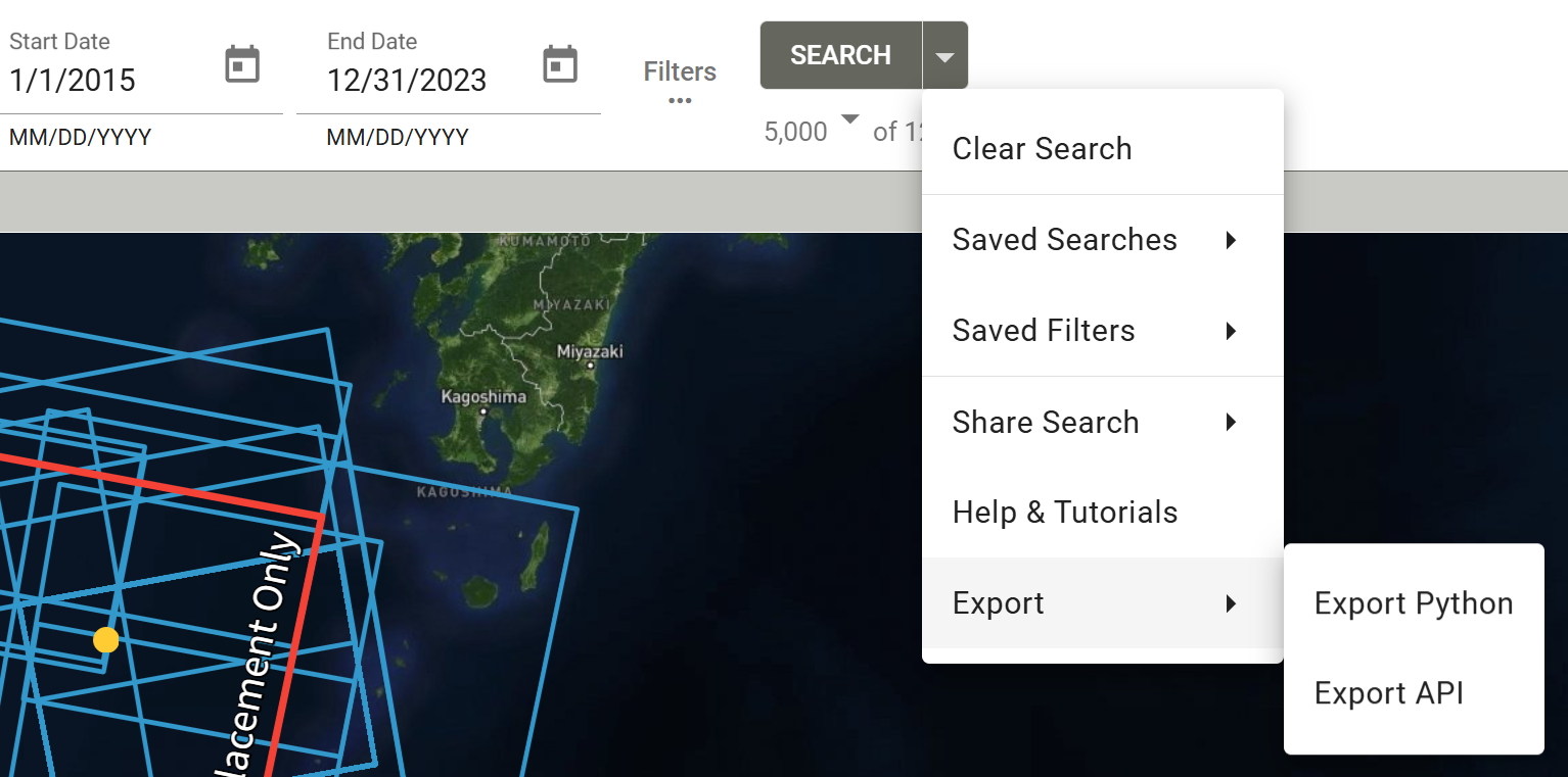
ASF Vertex: Export API - Click
Download Results.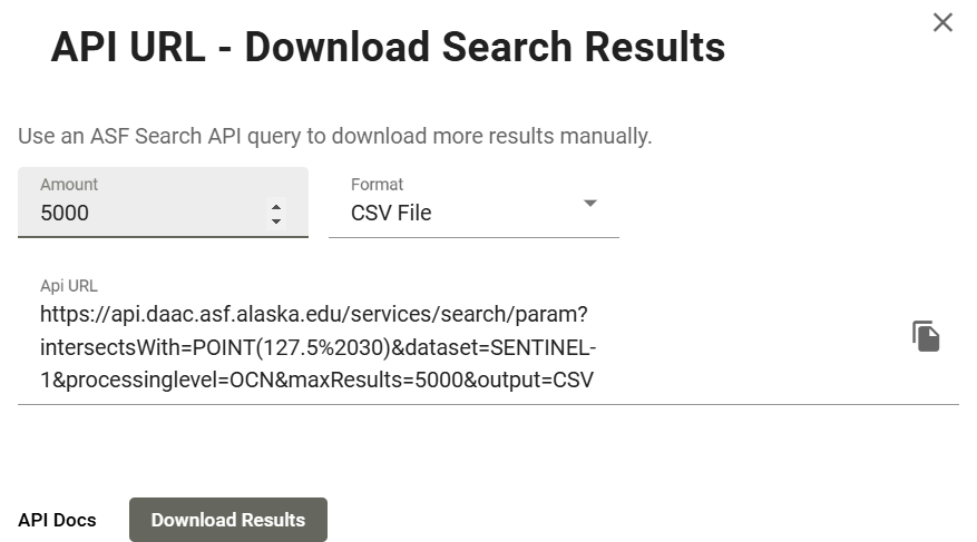
ASF Vertex: Download Results - Open the CSV. The
URLcolumn is what you need.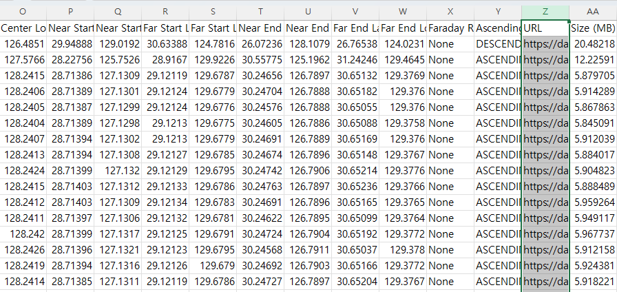
CSV exported from ASF with the URL column -
Run the MATLAB download loop below. You must be logged in to Earthdata before running it. It is a good idea to run the loop with
i=1only as a test: the Earthdata login page opens automatically, you log in there, and you can also check the download speed. If downloads are slow, increaselag_time.Open each ASF URL for downloadclc; clear; close all; % A file containing the data URL of the SAR satellite data downloaded % from the Alaska Satellite Facility (ASF) must be prepared read_xls; % read information about "URL" address in excel % Choose the appropriate value for your Internet speed environment lag_time = 1; % seconds between download each files. % Before executing the code, you must log in to the earthdata site in advance. % EARTHDATA Homepage : https://urs.earthdata.nasa.gov/ for i=1:length(URL) web(URL(i)) pause(lag_time); end -
The zip files are downloaded as shown.
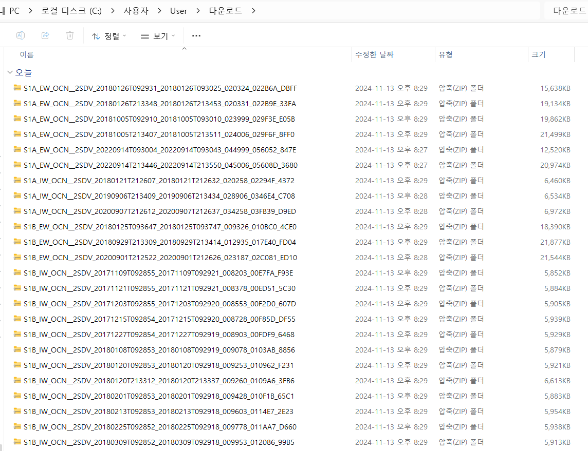
Downloaded zip files -
Unzipping by hand is tedious, so use MATLAB.
-
Visualization example.
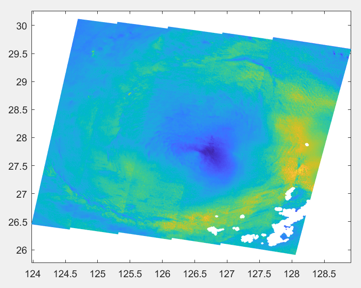
Sentinel-1 OCN wind speed plotted with pcolor Plot OCN wind speedclc; clear; close all; fnm = "C:\Users\User\OneDrive\문서\MATLAB\2024_Kuro" + ... "\khanun_SAR\S1A_EW_OCN__2SDV_20230804T213456_20230804T213559_049731_05FAEB_00F4.SAFE" + ... "\measurement\s1a-ew-ocn-vv-20230804t213456-20230804t213559-049731-05FAEB-001.nc"; wind = ncread(fnm, 'owiWindSpeed'); lon = ncread(fnm, 'owiLon'); lat = ncread(fnm, 'owiLat'); figure pcolor(lon, lat, wind); shading interp
Download ERS SAR data
Download Sentinel-1 from Copernicus Data Space
- Open the Copernicus Data Space Ecosystem and register.
- Click the green
Copernicus Browserbutton at the top right.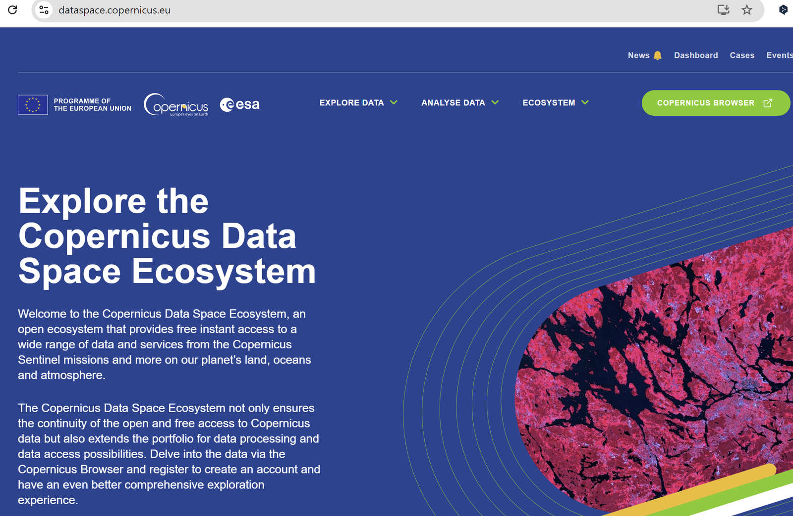
Copernicus Data Space: Copernicus Browser button 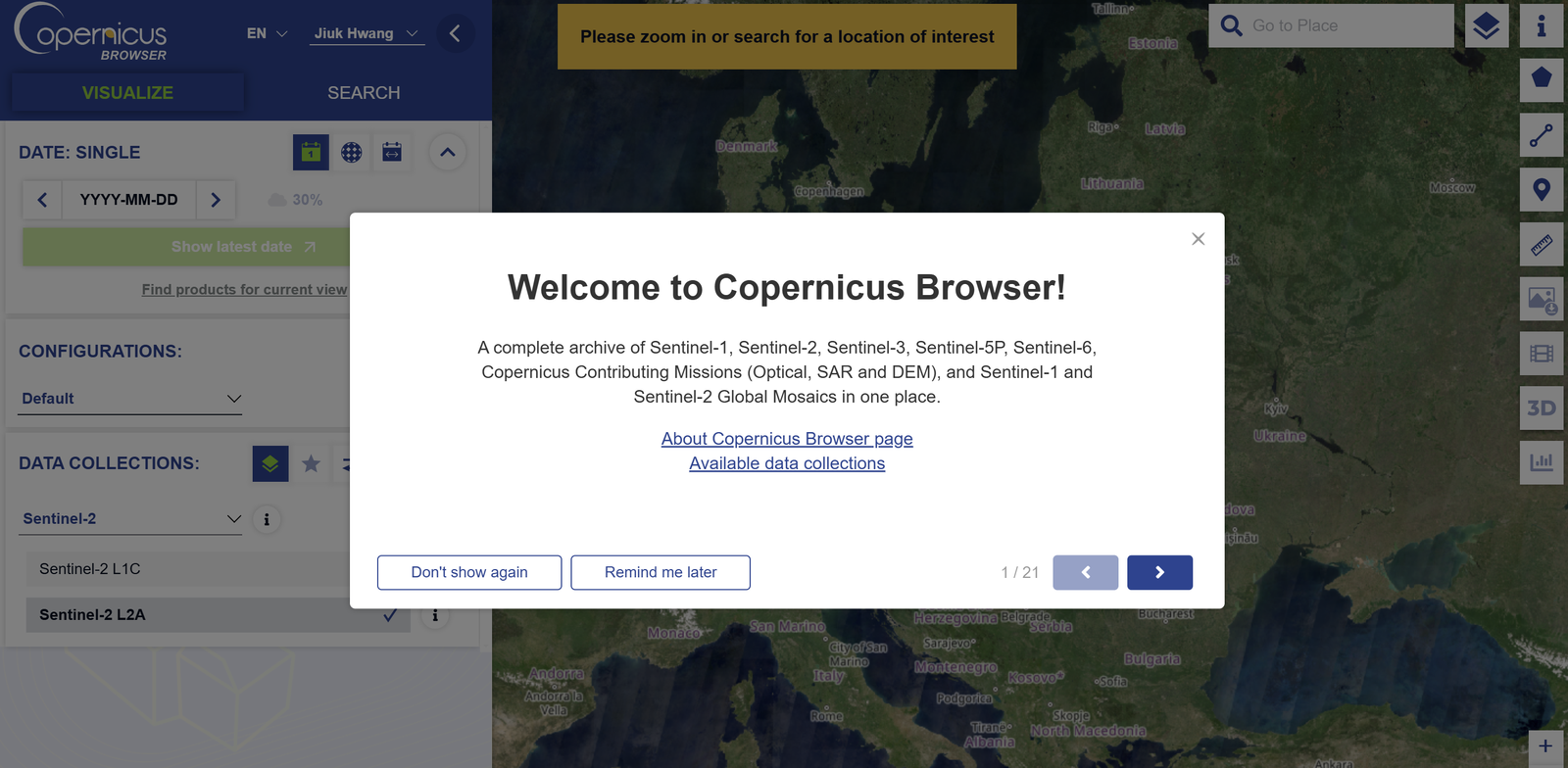
Copernicus Browser - In the
SEARCHpanel choose the satellite and product, then click the greenSearchbutton at the bottom. For a class assignment, Level-1 GRD > IW > VV+VH or HH+HV was used.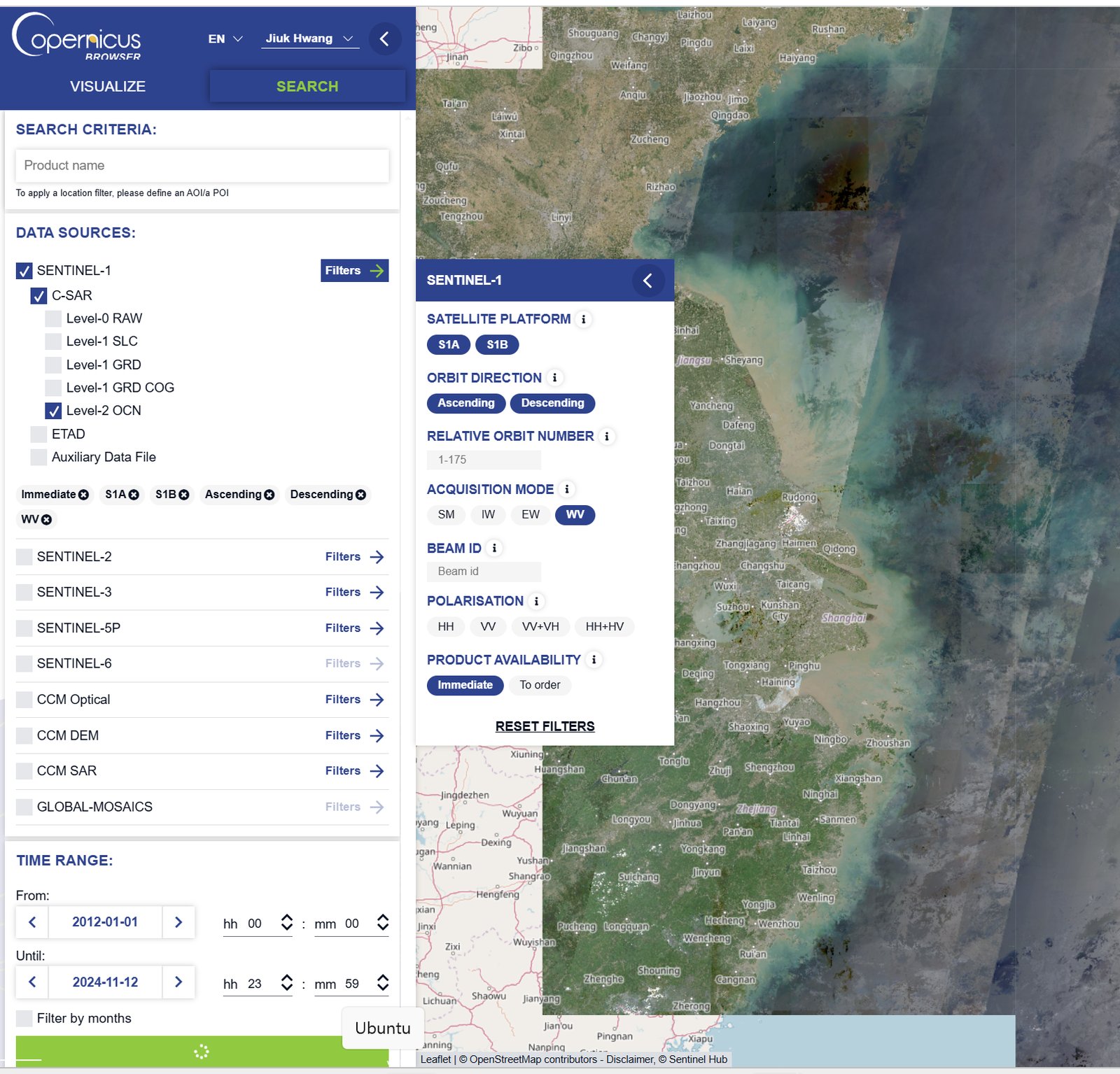
Copernicus Browser: search settings - Data for a specific date can be downloaded.
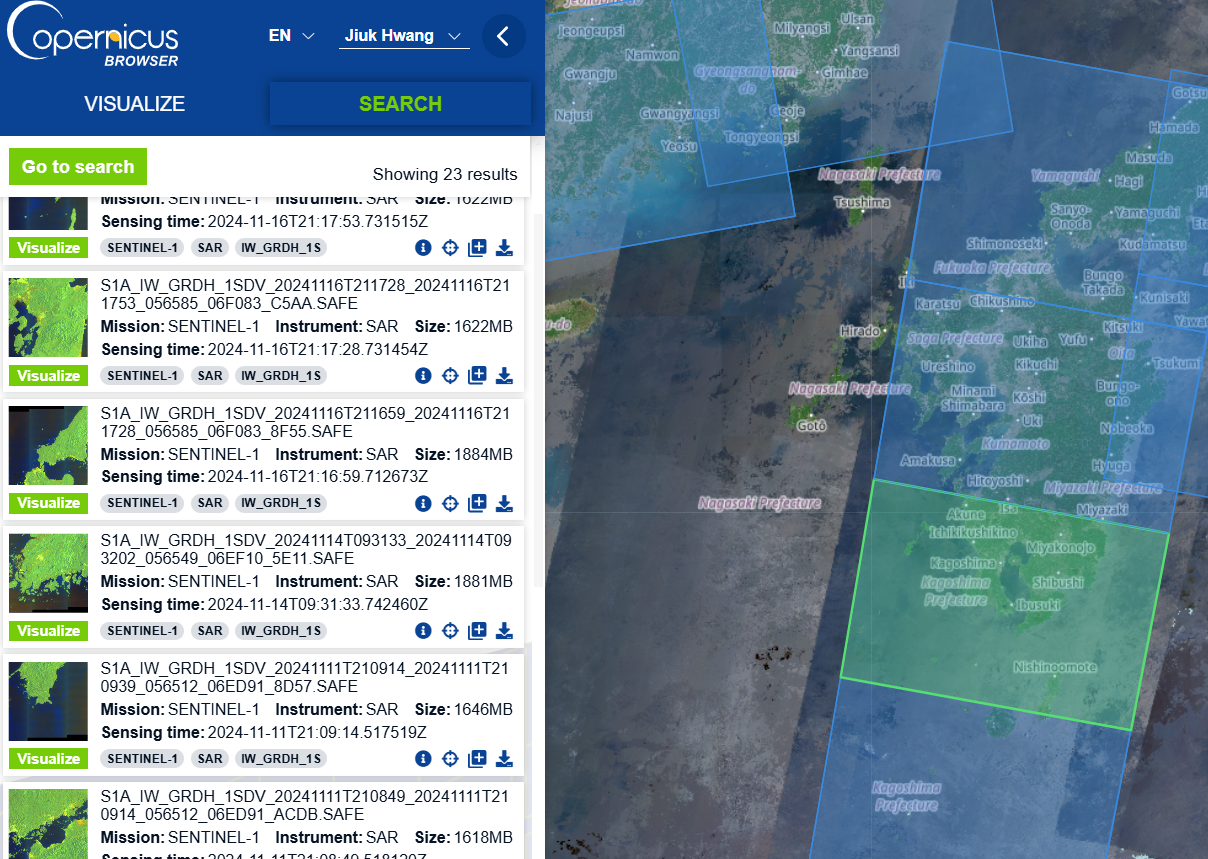
Copernicus Browser: search results 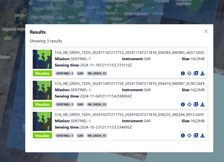
Copernicus Browser: download - Many scenes over a long period and a wide area can be downloaded at once from the data workspace.
Sentinel-6A altimetry (PO.DAAC)
- Sentinel-6A MF Jason-CS L3 P4 Altimeter HR NTC Ocean Surface Topography, F08
- Sentinel-6A MF Jason-CS L3 P4 Altimeter LR NTC Ocean Surface Topography, F08
Sea state from Sentinel-1 (Ifremer)
- umr-lops/sarwaveifrproc: processor that generates Level-2 WAV sea-state products from Sentinel-1 SAR (UMR LOPS)